Handling time data in buzzr
time-interpretation.RmdPassive monitoring goes hand-in-hand with (i) large datasets and (ii) long datasets. By which I mean, you probably have (i) lots of files/folders, and they (ii) span long stretches of time. With active observation, you’re probably finishing up a round of data collection within one day (even if you’re going back the next). With passive observation, one file might capture more than one day of data and one folder might capture a week on a standard MP3 recorder or a month on a field recorder with a duty cycle. Thus, tracking time is an essential component of a passive acoustic monitoring pipeline.
TL;DR
buzzr can automatically interpret the start time of audio files based
on their name, if a timestamp is used in the file name. This feature is
baked into the read_ functions and anything that calls
them, notably: read_results(),
read_directory(), and bin_directory(). Pass
the POSIX format code (see base::format.POSIXct()) to the
posix_formats argument as well as a time zone to
tz; buzzr will translate the file-time (seconds) to a
date-time (year, month, day, hour, minute, second). You can even pass
multiple format codes if you have mixed timestamps in your dataset!
Warning: Date coercion could drive you insane
Any time you’re working with POSIXct (that is, date-time) data, write to .rds files using saveRDS. Do not save date-times to .csv files.
POSIXct data are numeric under the hood, even though we write them as text. “August 8, 2023 12:34 PM” has the value 1,691,598,840.
"2023-08-09 12:34:00 EDT" |>
  as.POSIXct() |>
  as.numeric()
#> [1] 1691584440
It’s that many seconds from the start of the Unix Epoch. So, when you want to write it to a .csv file, R has to take a stab at formatting the numeric into text. When the POSIXct time corresponds exactly to midnight, R formats it without any hour, minute, or second. That is, just a date.
"2023-08-09 12:34:00 EDT" |>
  as.POSIXct() |>
  format()
#> [1] "2023-08-09 12:34:00"

"2023-08-09 00:00:00 EDT" |>
  as.POSIXct() |>
  format()
#> [1] "2023-08-09"
When R reads that CSV back in and you try to turn the column into date-times, if it sees any value that’s just a date, it will turn the entire column into dates.
c("2023-08-09 15:24:57 EDT", "2023-08-09", "2023-08-09 12:34:00 EDT") |>
  as.POSIXct()
#> [1] "2023-08-09 UTC" "2023-08-09 UTC" "2023-08-09 UTC"
Avoid this by using .rds files, which save the full time information. When you read in a .rds file, you get back exactly the same object you wrote. And they’re smaller and they’re faster! Friends don’t let friends comma-separate.
Types of time
buzzr works with two different representations of time:
-
File-time (column:
start_filetime): seconds elapsed since the start of the audio file. This is present in the raw buzzdetect results files asstart. -
Date-time (column:
start_datetime): a real-world timestamp, e.g.2023-08-09 06:00:00. To get this, buzzr needs to know when the recording started, which it reads from the file name.
This vignette explains how buzzr converts file names into date-times, how to handle mixed patterns in filenames (e.g. from different recorder types), and how to work with the resulting timestamps for plotting and modelling.
Reading a timestamp from a file name
Most field recorders embed the recording start time in the file name.
buzzr reads this using the same POSIX format codes as base R’s
strptime(). For example, you might see:
| File name | Format string |
|---|---|
230809_0000 |
'%y%m%d_%H%M' |
20230809_000000 |
'%Y%m%d_%H%M%S' |
2023-08-09_00-00-00 |
'%Y-%m-%d_%H-%M-%S' |
The Five Flowers dataset included with buzzr uses the
YYMMDD_HHMM pattern, since that’s what our (the Ohio State
University Bee Lab) recorders (Sony ICD-PX370) use. Let’s parse a single
file:
path <- system.file(
  'extdata/five_flowers_snip/soybean/53/230809_0700_buzzdetect.csv',
  package = 'buzzr'
)

# Without posix_formats: time stays as file-time (seconds from file start)
head(read_results(path), 3)
#>    start_filetime activation_ins_trill activation_mech_plane
#>             <num>                <num>                 <num>
#> 1:           0.00                 -2.3                  -1.9
#> 2:           0.96                 -2.6                  -2.7
#> 3:           1.92                 -2.2                  -2.4
#>    activation_ambient_rain activation_ins_buzz
#>                      <num>               <num>
#> 1:                    -1.7                -1.9
#> 2:                    -2.9                -2.2
#> 3:                    -2.5                -2.0

# With posix_formats: file-time is converted to an absolute date-time
head(read_results(path, posix_formats = '%y%m%d_%H%M', tz = 'America/New_York'), 3)
#>         start_datetime activation_ins_trill activation_mech_plane
#>                 <POSc>                <num>                 <num>
#> 1: 2023-08-09 07:00:00                 -2.3                  -1.9
#> 2: 2023-08-09 07:00:00                 -2.6                  -2.7
#> 3: 2023-08-09 07:00:01                 -2.2                  -2.4
#>    activation_ambient_rain activation_ins_buzz
#>                      <num>               <num>
#> 1:                    -1.7                -1.9
#> 2:                    -2.9                -2.2
#> 3:                    -2.5                -2.0
You can also call file_start_time() directly if you just
want the recording’s start time without reading the full file:
file_start_time(path, posix_formats = '%y%m%d_%H%M', tz = 'America/New_York')
#> [1] "2023-08-09 07:00:00 EDT"
Additional characters in the filename probably won’t mess up the extraction as long as they don’t also match the timestamp pattern.
buzzr::file_start_time(
  'tmp_230809_1359_corrected_bad_time_whoops_buzzdetect.csv',
  posix_formats = '%y%m%d_%H%M',
  tz = 'America/New_York'
)
#> [1] "2023-08-09 13:59:00 EDT"
Time zones
You must always pass a tz argument. Time zones are a
nightmare and they will bite you. To minimize our culpability,
we try to make buzzr utterly explicit about time zones. In general, it
will never guess and will always ask. The exceptions are
commontime() , which defaults to your local time zone since
it destroys relevant time zone information, and
label_hour() which interacts with
ggplot2::scale_x_datetime(), which guesses your time zone
anyways.
Use OlsonNames() to browse valid time zone strings.
Keeping both time columns
By default, start_filetime is dropped once
start_datetime is added. Set
drop_filetime = FALSE to keep both:
head(
  read_results(
    path,
    posix_formats = '%y%m%d_%H%M',
    tz = 'America/New_York',
    drop_filetime = FALSE
  ),
  3
)
#>         start_datetime start_filetime activation_ins_trill
#>                 <POSc>          <num>                <num>
#> 1: 2023-08-09 07:00:00           0.00                 -2.3
#> 2: 2023-08-09 07:00:00           0.96                 -2.6
#> 3: 2023-08-09 07:00:01           1.92                 -2.2
#>    activation_mech_plane activation_ambient_rain activation_ins_buzz
#>                    <num>                   <num>               <num>
#> 1:                  -1.9                    -1.7                -1.9
#> 2:                  -2.7                    -2.9                -2.2
#> 3:                  -2.4                    -2.5                -2.0
File-time can be useful if you want to reference the audio that corresponds to certain events. For example, you could use FFmpeg to extract the most active 5 minutes from every recorder or pull out every positive frame to review.
Multiple timestamp formats
If your experiment used more than one type of recorder, the file names may follow different timestamp conventions.
# Imagine two recorder types in the same experiment:
#   AudioMoth:  YYYYMMDD_HHMMSS  e.g. 20230809_060000_buzzdetect.csv
#   Sony:  YYMMDD_HHMM      e.g. 230809_0600_buzzdetect.csv

paths_mixed <- c(
  'site_a/audiomoth/20230809_060000_buzzdetect.csv',  # AudioMoth
  'site_b/Sony/230809_0600_buzzdetect.csv'       # Sony
)
buzzr can handle this, just supply all audio formats to the posix_formats argument. When each file matches exactly one format, everything resolves cleanly:
formats_mixed <- c('%Y%m%d_%H%M%S', '%y%m%d_%H%M')

file_start_time(paths_mixed, posix_formats = formats_mixed, tz = 'America/New_York')
#> [1] "2023-08-09 06:00:00 EDT" "2023-08-09 06:00:00 EDT"
When a timestamp matches multiple formats
This is where things get tricky. A Sony file like
230809_0600 is YYMMDD, but perhaps another recorder has a
format of YYDDMM. Or, maybe you’re using an AudioMoth recorder that
includes the seconds count and you want accuracy down to the second.
Since you can’t parse seconds from the Sony file name, those dates would
fail.
By default (first_match = FALSE), buzzr returns
NA and warns you when formats conflict:
# Construct a path that matches both formats ambiguously
ambiguous_path <- 'site/recorder/20230809_060030_buzzdetect.csv'

file_start_time(
  ambiguous_path,
  posix_formats = c('%Y%m%d_%H%M%S', '%y%m%d_%H%M'),
  tz = 'America/New_York',
  first_match = FALSE
)
#> Warning: Returning NA for start time of file 'site/recorder/20230809_060030_buzzdetect.csv'; multiple POSIX matches:
#> %Y%m%d_%H%M%S
#> %y%m%d_%H%M
#> [1] NA
If you set first_match = TRUE, formats will be matched
in the order they appear, accepting the first matching format and moving
on even if later formats match, too:
file_start_time(
  ambiguous_path,
  posix_formats = c('%Y%m%d_%H%M%S', '%y%m%d_%H%M'),
  tz = 'America/New_York',
  first_match = TRUE
)
#> Multiple POSIXct patterns match for file 'site/recorder/20230809_060030_buzzdetect.csv'. Accepting first: %Y%m%d_%H%M%S
#> [1] "2023-08-09 06:00:30 EDT"

# Swap the order — now the seconds aren't extracted from the filename
file_start_time(
  ambiguous_path,
  posix_formats = c('%y%m%d_%H%M', '%Y%m%d_%H%M%S'),
  tz = 'America/New_York',
  first_match = TRUE
)
#> Multiple POSIXct patterns match for file 'site/recorder/20230809_060030_buzzdetect.csv'. Accepting first: %y%m%d_%H%M
#> [1] "2023-08-09 06:00:00 EDT"
When a file matches two formats with the same result
Even with first_match=FALSE, if multiple formats resolve
to an identical timestamp, buzzr silently deduplicates:
# These two formats both parse '230809_0600' as 2023-08-09 06:00:00
file_start_time(
  'site/recorder/230809_060000_buzzdetect.csv',
  posix_formats = c('%y%m%d_%H%M', '%y%m%d_%H%M%S'),
  tz = 'America/New_York',
  first_match=FALSE
)
#> [1] "2023-08-09 06:00:00 EDT"
Since the seconds really are zero, both formats gets the same answer and buzzr accepts it without a message. This is pretty common if your field recorders are starting on the minute.
If no format matches
buzzr returns NA with a warning, so downstream code
doesn’t fail silently:
file_start_time(
  'site/recorder/no_timestamp_here_buzzdetect.csv',
  posix_formats = '%y%m%d_%H%M',
  tz = 'America/New_York'
)
#> Warning: Returning NA for start time of file
#> 'site/recorder/no_timestamp_here_buzzdetect.csv'. No POSIX matches found.
#> [1] NA
Time of day for modeling: time_of_day()
When doing stats on time of day, you probably don’t want to use a POSIXct object. For one thing, your coefficient values will have units of seconds, which is unlikely to be informative. For another, if your recordings were conducted on different days, you need to tell the model to ignore the date.
buzzr::time_of_day() is a very simple convenience
function that returns either a proportion of the 24-hour day or a
decimal hour:
times <- as.POSIXct(
  c('2023-08-09 00:00:00', '2023-08-09 06:00:00',
    '2023-08-09 12:00:00', '2023-08-09 18:30:00'),
  tz = 'America/New_York'
)

# Proportion: midnight = 0, noon = 0.5, next midnight = 1
time_of_day(times)
#> [1] 0.0000000 0.2500000 0.5000000 0.7708333

# Decimal hours: midnight = 0, 6 AM = 6, 6:30 PM = 18.5
time_of_day(times, time_format = 'hour')
#> [1]  0.0  6.0 12.0 18.5
Time of day for plotting: commontime(),
label_hour()
It’s often annoying to plot date times. We might want to compare
daily trends, so we use time on the X axis. But if your recordings were
conducted on different days, they won’t overlap. We could use a solution
like time_of_day(), but then our X axis is funky; who wants
to see X=0.77 on a diel plot?
commontime()solves this by setting every date to the
same arbitrary day (2000-01-01) while preserving the hour, minute, and
second and leaving the class as POSIXct. This allows us to make pretty X
axis labels using ggplot2::scale_x_datetime() and another
buzzr function, label_hour()/
dir <- system.file('extdata/five_flowers', package = 'buzzr')

binned <- bin_directory(
  dir_results   = dir,
  thresholds    = c(ins_buzz = -1.2),
  posix_formats = '%y%m%d_%H%M',
  tz            = 'America/New_York',
  dir_nesting   = c('flower', 'recorder'),
  binwidth       = 20,
  calculate_rate = TRUE
)
#> Grouping time bins using columns: flower, recorder

# Dates vary across the five recordings; commontime collapses them
range(binned$bin_datetime)
#> [1] "2023-08-09 00:00:00 EDT" "2025-07-04 23:40:00 EDT"

binned$time_of_day <- commontime(binned$bin_datetime, tz = 'America/New_York')
range(binned$time_of_day)
#> [1] "2000-01-01 00:00:00 EST" "2000-01-01 23:40:00 EST"
Now all five flowers share the same x axis, regardless of which day they were recorded:
library(ggplot2)

ggplot(binned, aes(x = time_of_day, y = detectionrate_ins_buzz, color = flower)) +
  geom_line() +
  scale_x_datetime(labels = buzzr::label_hour(tz = 'America/New_York')) +
  labs(x = 'Time of day', y = 'Detection\nrate', color = 'Flower') +
  theme_buzzr()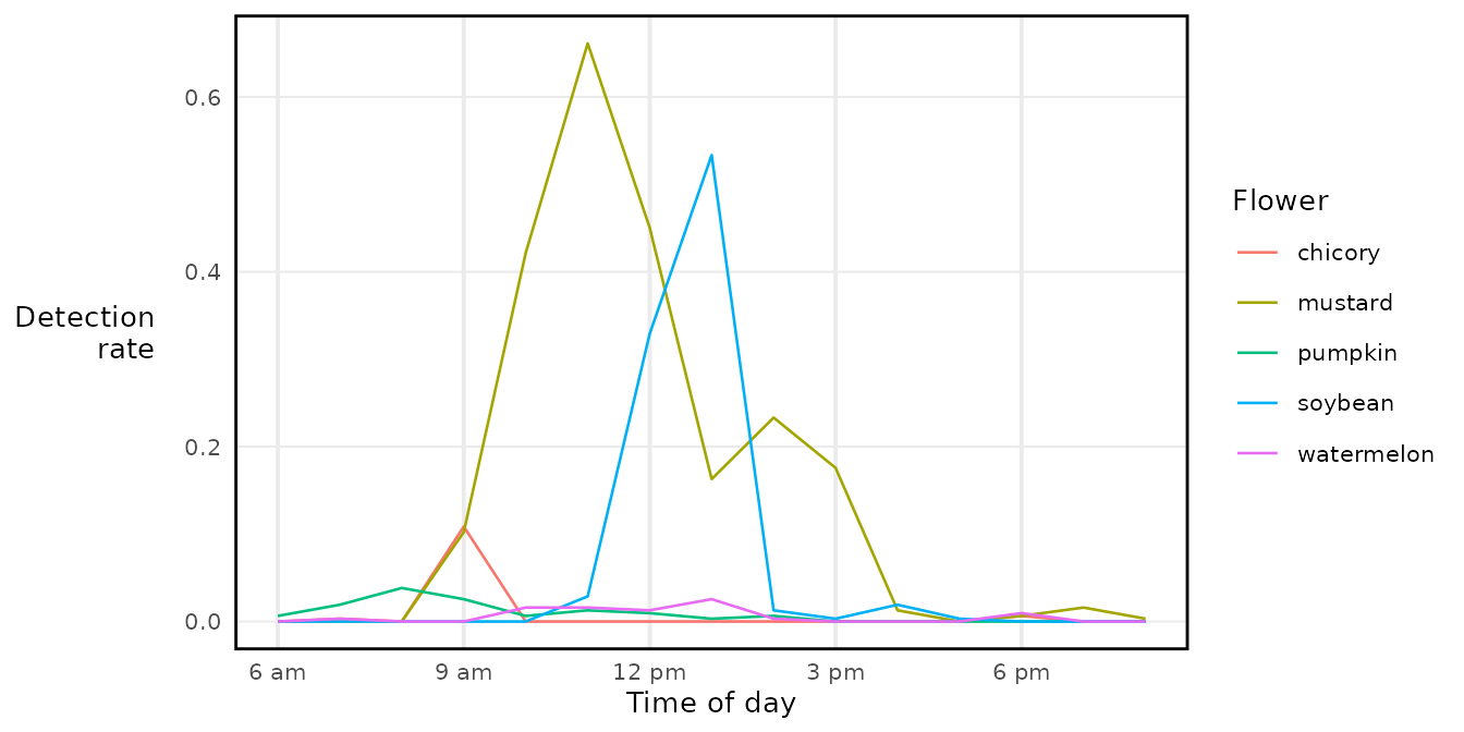
Always pass the same tz to commontime() and
label_hour(). If they differ, the axis labels won’t match
the data.